Lowest Total Cost of Inventory

Calculating the cost of holding inventory is typically not available in supply chain applications. But this is one of the required inputs for establishing and maintaining an Inventory Policy.

Approaches to determining the amount of inventory needed to satisfy customer expectations range from a ‘rule of thumb’ approach such as ‘order X weeks of stock when the amount on hand is Y weeks of stock’, to complex simulations. These endeavour to replicate real world uncertainty concerning the demand per period, supply lead time and other relevant factors that may exhibit variability.

However, these methods rarely address the total cost, especially where there may be potential for significant amounts of unsaleable stock due to the expiry date, or lost sales due to non-availability to meet demand.  For short shelf-life products in particular, these costs can be substantial.

Stock Optimiser v2

David Cobby has developed a solution to this challenge. Stock Optimiser is a Microsoft Excel tool for determining the lowest total cost of carrying inventory.

The Stock Optimiser Excel spreadsheet is attached. The tool seeks to obtain the best overall cost solution, using optimisation within an Excel model that incorporates the Solver functionality. 

Accessing Solver

Solver is an add-in to Excel, but is not enabled. To load Solver in Excel 2019:

• In Excel click the File Tab
• Go to Option at bottom of the File list
• Click Options
• Select Add-ins from the list
• Select Solver Add-in from the list of Application Add-ins
• Ensure that a tick mark is displayed and click OK to exit the list
• Return to the Data tab; Solver should be available in the Analyze section

Objective of Stock Optimiser

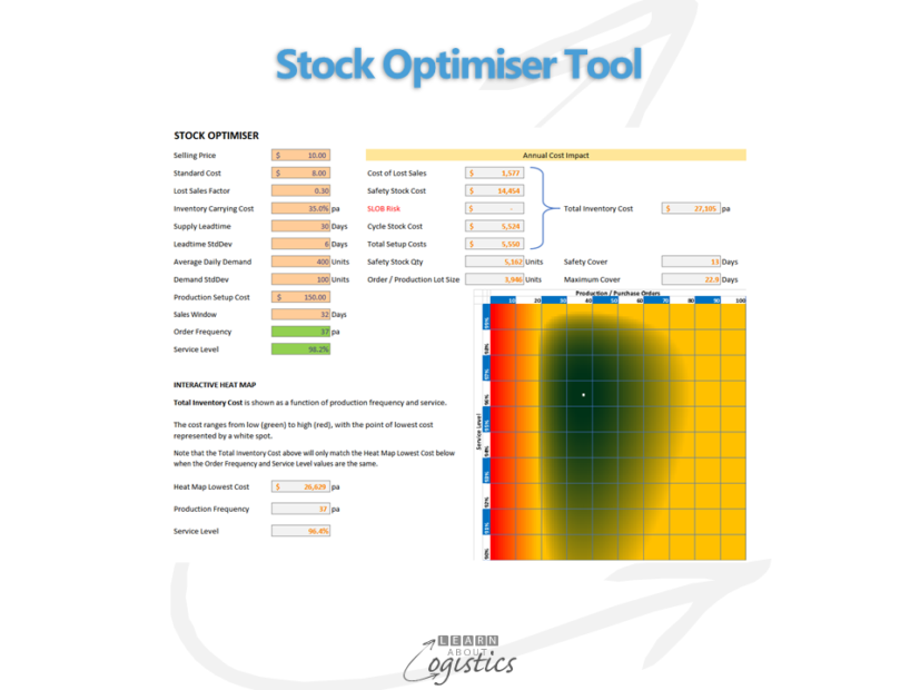
The tool enables a balance to be obtained between the frequency of replenishment (or order lot size) against the service level provided, using the following elements:

• impact of lost sales
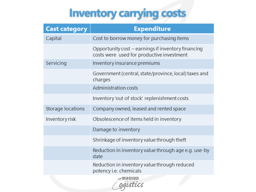
• inventory carrying cost
• average supply lead time and its variability
• average demand and its variability
• ordering or production setup cost
• selling window (for perishable products, the difference between shelf life at the time of release from manufacturing for sale and the minimum shelf life required by customers)

A Heat Map is included, to assist your understanding concerning the impact for different elements of the model on total cost. This covers the service level range of 90 percent or greater and 0 to 100 orders per annum.  The Heat Map can be used interactively to evaluate how a change to one of the input values affects the Total Inventory Cost.

Note: The calculations are based on average daily demand over 365 days.  These can be changed to reflect the number of trading days over a year.  The Heat Map worksheet will then require the formulas in each cell to be adjusted.

Principles underlying the worksheet calculations

• Cost of Lost Sales is the loss of gross profit incurred over a year for the designated level of un-serviced demand (100% less the designated service level)
• Safety Stock Cost calculation uses the well-known statistical safety stock formula. Other calculations such as risk of a stock outage over the lead time could also be employed
• SLOB (slow and obsolete) Risk calculation is intended for use with products that have a shelf life, based on the number of selling days before the product reaches the minimum remaining shelf life that is acceptable to customers.  This is not the actual SLOB that will be incurred, but rather an indicator of the relative impact of a set of values versus another set (for example the effect of a significant change in demand variability represented by the demand standard deviation).  Normally, a business will actively pursue opportunities to mitigate its risk of unsaleable product by seeking alternative sales avenues, discounting etc.
• Cycle Stock Cost is the carrying cost for the average quantity of cycle stock on hand
• Total Setup Cost is the number of production orders per annum multiplied by the cost of a setup
• Total Inventory Cost is the addition of the five elements described above

User Input Elements

Most of the elements are self-explanatory (based on the names applied to them) and are usually available in a business.  These elements do not normally vary significantly in the short term.

Terms that may require some clarification are:

• Lost Sales Factor is a notional effect on sales of not having an item when demanded by a customer.  If customers are unwilling to wait for the item and instead buy from a competitor (zero brand loyalty and / or the product is considered a commodity), the lost sales factor would be 1.0 (possibly higher if the item is subject to repeat purchase by a customer and there is evidence that repeat sales would be lost).  At the other extreme, if all potential customers are prepared to wait, the factor would be zero (applicable for products with extreme brand loyalty).  This effectively makes customer service irrelevant to cost over a range of service levels.  In cases where it can be difficult to assess the lost sales factor, use a value of 0.5.
• Inventory Carrying Cost is the percentage overhead (or burden) applied to an item for holding it in inventory.  This should comprise only those cost elements that are proportional to the amount of inventory.

Production Setup Cost should account for variable cost elements only, such as consumables and production waste incurred during setup.  Any dedicated resources that only perform setup related activities are treated as fixed costs.

The Heat Map

This is a three-dimensional chart with the cost (third dimension) represented by colour (green is low cost and red is high), with the lowest cost point being the white spot.  The Heat Map is an embedded image on the Stock Optimiser worksheet.

Changing the values in the pink shaded cells will result in the colours shifting and white spot moving.  In some rare circumstances there will be no apparent change and in others, the white spot may change to a white line or larger white area.  These are not errors, but rather special cases, where costs have shifted uniformly up or down (i.e. no apparent changes) or there are multiple points of lowest cost as can occur if there is no Lost Sales Factor and a high Production Setup Cost.

Note: the map operates independently of Solver and the values in green shaded Production Frequency and Service Level cells.  To make the calculations (the cells containing orange values) reflect the lowest cost point in the Heat Map, change the Production Frequency and Service Level values in the green shaded cells to match the orange values at bottom left of the Heat Map. 

Note: the Heat Map approach only considers Service Level to a single decimal place, so it will generally return a slightly different result to Solver.

The Heat Map can be an effective way of demonstrating the inventory cost impact of each parameter in the model; so spend time trying different values in the various fields. By incrementally changing only one value in the pink shaded cells, it is possible to see how the shape of the map changes and the lowest cost point moves.

For example, start with a Demand StdDev that is small relative to the Average Daily Demand, then gradually increase it while observing the SLOB Risk value.  Notice how the SLOB Risk rapidly increases once it comes into play, due to the demand variability.

Note: Solver run times can be adversely impacted by the Heat Map image on the Stock Optimiser worksheet. Therefore, make a copy of the spreadsheet with a different name and delete the Heat Map image in the version that will use Solver.  This will not affect the main Heat Map.

Setting Order Frequency and Stock Availability Service Level Limits

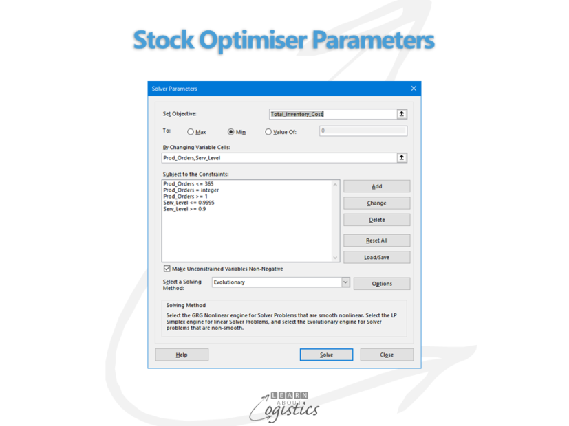
In determining the best cost solution, Solver varies the orders per annum and service level over user defined ranges until the lowest total cost is found. Note this may not be the absolute ‘best’ cost, due to the limits imposed by the user. This will be evident if either the number of production orders or the service level returned as results is the same as one of the upper or lower limits imposed in Solver.

Setting the limits.

1. Open the Solver dialog window (see below).  The large box in the middle of this window named Subject to the Constraints shows several lines with range names and values separated by <=, = or >=.  These are the limits imposed on Solver when seeking the best outcome for the objective value (in this case, the Total_Inventory_Cost value in the Set Objective field).

2. Select the item you want to modify and click Change.  The Change Constraint window will open as below.

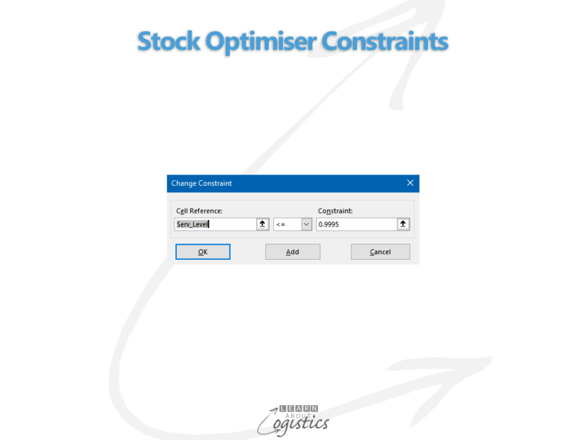
3. Select the item you want to modify and click Change. The Change Constraint window will open as below.

Note: Do NOT modify the Solving Method and Options. These have been set to reflect the characteristics of the model and generate a realistic solution within a reasonable time. 

The Set Objective box must NOT be changed from Total_Inventory_Cost.

Our thanks to David for making his inventory tool available. It will be useful when setting the Inventory Policy for your business and valuable when explaining the value of inventory to senior executives.