Actions to limit variability

Increasing numbers of stock keeping units (SKUs), extended and variable lead times and shorter planning horizons are challenges for planners. Variability was discussed in the previous blogpost, identifying (at the end) actions that could be taken to limit variability.

One action is to manage the allocation of finite capacity within a business. An approach to increasing the capacity available is through Assets Support Logistics, incorporating Overall Equipment Efficiency (OEE). This is discussed in the blogpost Assets Support Logistics role in achieving Availability

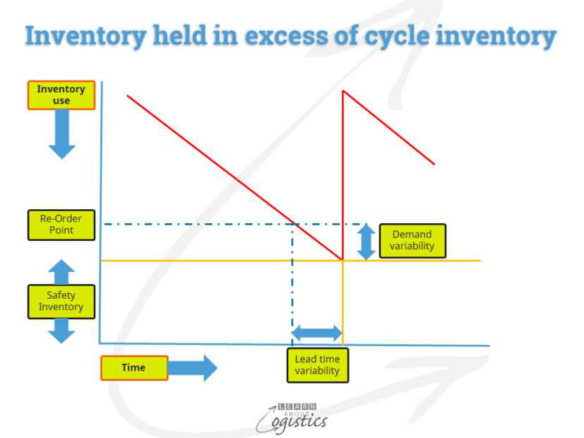
The other action is providing Safety Inventory to cover the calculated variability in supply lead times and the difference between the order interval and the delivery lead time.

The diagram below illustrates inventory variability. Safety Inventory is held in excess of the cycle inventory (inventory held at the mid-point through the replenishment cycle – half the order quantity) to address the uncertainty associated with unplanned events – that is variability. Safety inventory can also be called safety stock, reserve stock or buffer stock.

Demand Management is the responsibility of Marketing and Sales. The Sales and Operations Planning (S&OP) process is the structure used for linking the Demand and Supply Plans. Demand Management has three core elements:

• Demand Sensing: helps to identify buying trends for products, through analysing the data generated within each sales channel
• Demand Shaping: incentive programs designed to increase customer and consumer demand for products 
• Demand Planning: builds sales forecasts from Demand Sensing and Shaping inputs. The factors affecting Demand variability are the mean of demand and forecast accuracy

Reducing supply variability

Supply variability is influenced by the mean lead time and lead time variability. If, in the replenishment period, there is an unplanned increase in demand and/or a longer lead time for the item, safety inventory will be used to satisfy the needs of customers. A role within Operations Planning (of resources and inventory) is to understand the reasons for and to influence the reduction in supply variability.

There are two calculations for the safety inventory required to cover variability in the lead times for SKUs.

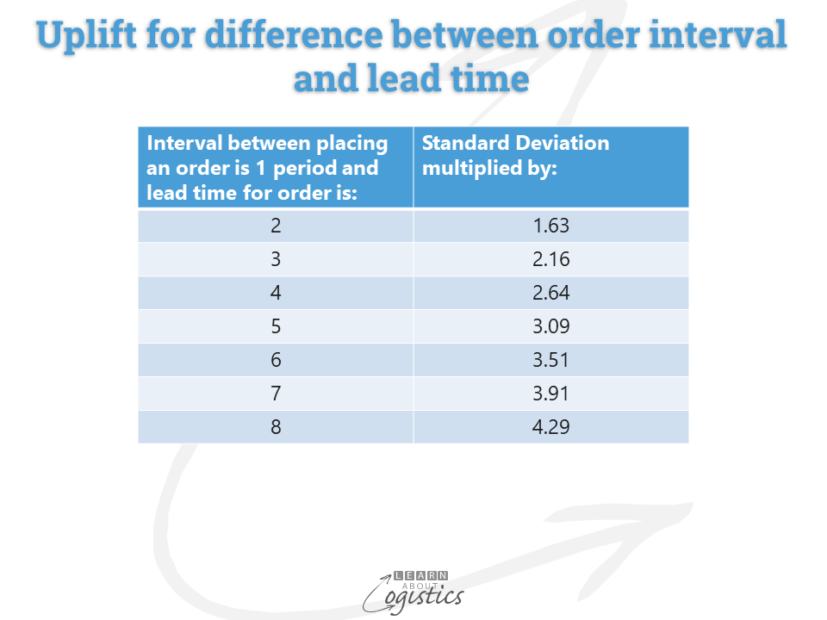
The first is to identify an uplift to the standard deviation of sales calculation for each SKU. Where the lead time to receive an SKU is more than the interval between placing orders, there is a likelihood that actual demand will differ from that forecast; so, the calculated standard deviation must be uplifted by a multiplier. This is shown in the table.

The second calculation is the variation in lead time between the planned and actual times. The calculation of safety stock for each SKU, to allow for variation in lead time (forecast LT against actual LT) is:

1. Standard deviation = Variance squared/periods
2. Square root of the period variance (rounded up)

The answer will provide safety inventory cover for an 84 per cent customer service level. This is in addition to the safety inventory calculated for cover for variation in demand and between the order period and delivery LT noted above. As the availability expectation is often to provide a 98 per cent service level, the total safety inventory for a SKU could be more than double the safety inventory required to cover just the demand variability.

Information required

As stated, calculating the safety inventory required to cover for variability is one of three variances. To establish the base information for calculating safety inventory requires an approach similar to that illustrated below, which is the matrix for placing SKUs by Category and Class.

The standard ABC analysis assumes the pattern of sales for the 15 – 20 percent of items in Category A (also items in Categories B and C) will be similar. Therefore all SKUs within the Category are treated the same, even though the pattern of demands will actually vary.

The Category breakdown for items is an example of a typical SKU list for a fast moving consumer goods (FMCG) or consumer packaged goods (CPG) business. The Class is calculated from the Coefficient of Variation (CoV) or (CV). This approach establishes the pattern of sales for SKUs within each Category, which can vary, requiring different approaches to forecasts and placing orders.

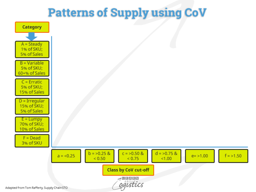
In statistics language, the Coefficient of Variation is a normalised measure of dispersion for a probability distribution; defined as the ratio of the standard deviation to the mean. The CoV for a SKU is calculated by dividing the standard deviation of sales for the SKU by its sales mean. The Class is identified by the CoV cut-off range. The range shown in the diagram is not definitive; in some organisations they limit ‘Class b’ to 0.3 and ‘Class d’ to 0.7.

The lower the CoV, the more consistent are sales and conversely, the higher the CoV, the greater the variability of sales for the SKU. Once plotted, the SKUs will have a pattern shown in the diagram, which by colour block relate to the Category names.

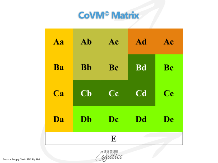
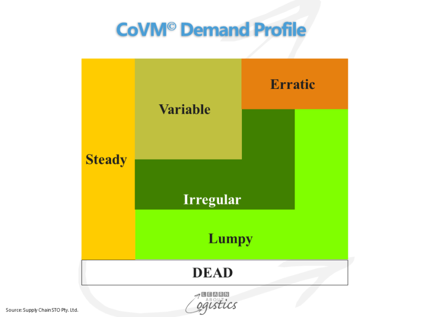
By placing the SKUs into their calculated cells in the matrix, it is evident that different inventory management approaches are required for each Category/Class, based on the pattern of demand:

• STEADY: the SKUs placed in ‘Class a’, where demand is steady with little variation, regardless of the volume sold or used
• VARIABLE: the variable sales pattern requires the calculated forecast error of the SKUs to be regularly reviewed
• ERRATIC: contains individual SKU items that have substantial sales, but sales volumes can vary dramatically. This is a challenge for logistics professionals, because the timing of a large sale may not be communicated
• IRREGULAR: usually purchased by customers in small quantities on an irregular basis. The number of SKUs in this group is similar to the total of the previous three groups, yet constitutes only about 10 per cent of sales
• LUMPY: can contain up to 70 per cent of all the SKUs, yet only about 5 per cent of the sales value – rarely ever more than 7 per cent
• DEAD: those SKUs are without any sales in the past 12 months

This discussion indicates that a Logistician requires the knowledge to structure an inventory matrix and sell the concept to corporate management. This will provide an incentive to minimise the variability (and safety inventory) in the system and to design and implement an inventory holding policy.