ABC inventory approach

Inventory is too often considered as one lump of cost, rather than as a collection of individual stock keeping units (SKUs), each with their own pattern of demand and supply.

To provide some differentiation between high and low selling items, a familiar process is to group SKUs into ABC groups. This is based on observations by the Swiss-based Italian economist Vilfredo Pareto in the early 1900s that about 80 per cent of influence in a situation is exerted by about 20 per cent of the elements involved. For example, 80 per cent of sales are made to 20 per cent of the customer base. This was later called the 80/20 rule or Pareto Principle.

The ABC analysis of finished goods is typically based on each SKU’s annual sales volume, calculated at the cost of goods sold (COGS) value. This removes the profit margin figure, which can bias results. To determine the ranking for each SKU:

• Multiply the annual sales volume of each SKU by its cost to manufacture or buy (COGS)
• Rank the SKUs by annual sales value, from highest to lowest
• Divide the annual value for each SKU by the inventory investment for all SKUs, to obtain percentage of the inventory investment for each SKU
• Cumulate the percentages, with cut-offs at about 80 percent, 90 percent and 95 percent. These are the A:B:C cut-offs. The breakdown can be extended to A:B:C:D groups

Improving the ABC approach

The limitation of constructing ABC groups is that all SKUs within a group are treated the same, even though their pattern of demand may vary. To overcome this limitation, the Coefficient of Variation (CoV) is calculated for each SKU and the result posted with the relevant Class cut-off, as shown on the right side in the Table below:

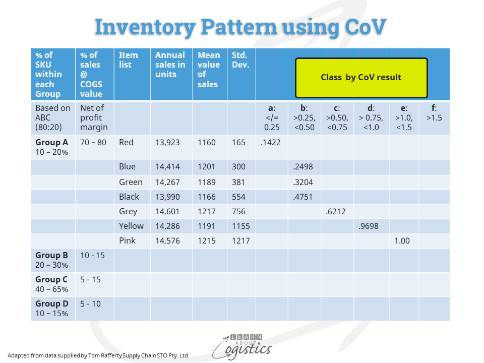
The layout of the Table shows on the left side, a breakdown of SKUs into groups A:B:C:D. Within Group A, seven SKUs have been identified by colour for a business and the annual sales listed for each SKU; this could be for the company or by location. As the annual sales figures are similar, it may be assumed that the sales behaviour of each SKU is the same, but this is not so.

The CoV is calculated by dividing the standard deviation for each SKU’s sales by the mean (average) sales. Following the CoV calculation, each SKU is allocated to its Class. The Table shows that SKU ‘Red’ is in ‘Class a’, three SKUs (Blue, Green, Black) are in Class b and one SKU in each of Class c, d and e.

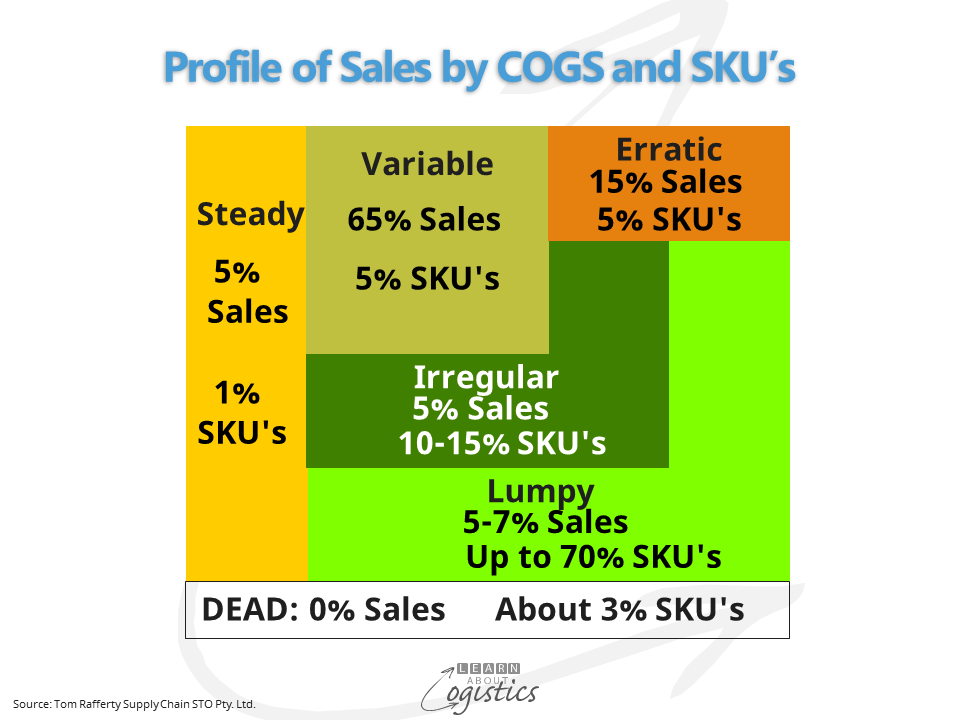
The SKUs in Group A can now be identified by their CoV Category/Class: Aa, Ab, Ac, Ad, Ae and if required, Af. It follows that SKUs within Groups B, C and D can also be allocated to a Class, which provides Category/Class Ba, Bb, Bc, Bd and Be and the same for SKUs within Groups C and D. As shown in the diagram below, the patterns of demand for each Category/Class are described as: Steady, Variable, Erratic, Irregular, Lumpy and Dead:

The weighting of each Category/Class by value and SKUs differs from the initial ABC calculation, as shown in the diagram below:

Inventory consultant, Tom Rafferty at Supply Chain STO Pty. Ltd. calls this approach CoV Management (CoVM), because the patterns of demand provides an indication of direction for managing inventory.

Actions to manage Inventory

No longer is there a need for the CEO to command “cut inventory by 10 percent”, or any other amount that sounds about right. The structured patterns of demand provide a format for ongoing actions by the organisation’s Supply Chains group; some of which are shown in the Table below:

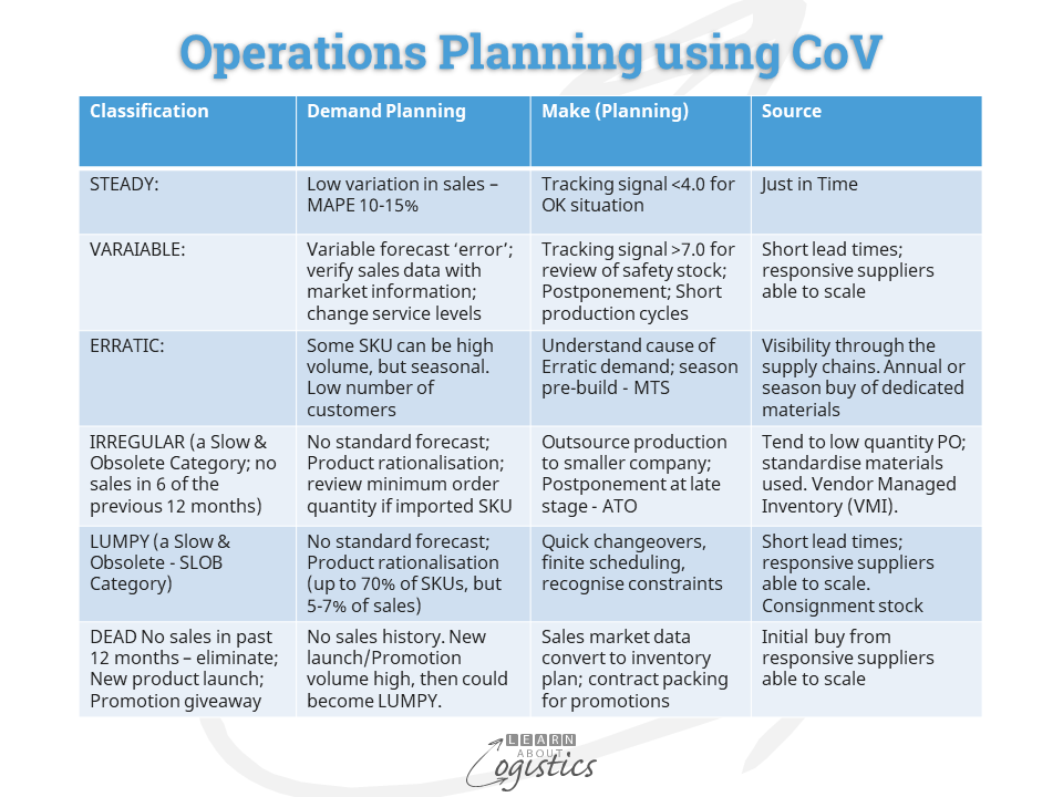
For STEADY and VARIABLE Category/Class, the mechanism for management is Tracking the accuracy of forecasts; this assumes that, regardless of volumes, demand has a low variation. As the SKUs are more likely Make to Stock (MTS), a high service level will not require a high physical safety stock.

The Tracking Signal is calculated as the Cumulative Variance (for each of the period’s between forecast and actual sales) divided by the Standard Deviation (calculated as the square root of the period variance average, which is the total of period variances squared, divided by the number of periods. For SKUs in the STEADY Category, a Tracking Signal of less than 4.0 indicates the forecasts for that SKU are in control. In the VARIABLE Category, the ‘forecast error’ will be higher. When the Tracking Signal exceeds 7.0, it is the trigger for a review of the forecast parameters, including the allocated service level.

SKUs in the ERRATIC Category can be a challenge for Logistics if they and Sales do not communicate concerning the timing of large orders (maybe seasonal) from customers. The Supply Chains group should understand the drivers for each customer pattern of orders for this Category/Class of SKUs.

The Slow and Obsolete (SLOB) Category/Class (IRREGULAR, LUMPY AND DEAD) often have too much inventory sitting in warehouses gathering dust and costing money. They cannot be forecast using standard time-series forecasting techniques, so excess safety stock is more likely, with associated inventory risks. New product launches, promotions and give-aways need to have the total cost identified and tracked by the Supply Chains group and Marketing/Sales. As Marketing usually resists the rationalising of product lines, the Supply Chains group must have a product line elimination strategy as part of the inventory management process.

Depending on the business and type of products, additional decision criteria may be used to place an SKU in its correct Category/Class. These include:

• total cost of ownership for the SKU
• total cost of a stock-out for the SKU (including reputational damage)
• product range integrity – to obtain the sale of a fast moving SKU, particular slow-moving items must also be available to make a ‘packaged’ sale. These assumptions must be evaluated
• physical size of the finished product
• risk of pilferage for the SKU or input materials
• shelf life and batch control requirements
• availability of specialist resources for the SKU to be produced
• storage requirements for finished products or materials e.g. very low temperature
• engineering or technical design complexity for SKU modifications
• high Procurement risks when obtaining materials or components

Inventory management is a critical concept in a logistician’s knowledge bank. It is about understanding and manipulating numbers and identifying patterns. CoV is a technique that provides many benefits, so it is of value to understand and use the approach for improved management of inventory.