Lead Time has a cost

Lead Time variability should be an important input for Operations Planning and Scheduling. However, although lead times are a factor in MRP calculations, few companies update lead times as they change, using the same values inputted when the ERP system was installed.

As discussed in the previous blogpost, the lead time from a supplier is not critical if orders and shipments are on a regular basis and the times are adhered to. However, if there is variability in the lead times, action must be taken. An example is a supplier of a critical item showing a trend towards delays in deliveries, so the timing of order placement must be adjusted. Unfortunately, planning applications are rarely designed to track lead time variability, while reorder points and order quantities do not adapt with changing lead time variability and patterns of consumer demand.

Within the Supply Chains group, Procurement negotiates the lead times within a contract, Logistics is responsible for influencing a reduction in lead times and their variability and Operations Planning identifies the current lead times and variability to apply within the Sales & Operations Planning (S&OP) process and when scheduling Operations. However, as more data becomes available, predictive analysis will enable processes to be improved that (hopefully) will limit the impacts of variability.

For the Supply Chains group, a greater degree of Uncertainty exists with longer and more variable lead times, such as forecast ‘errors’ that are amplified by lead time variability. And, Uncertainty equates to Supply Chains Risk. When a buyer places an order for a product or an item, a financial exposure occurs and therefore risk. The value of risk exposure is measured by Inventory Exposure, which represents the total amount of money committed (although not necessarily paid) and therefore at risk at a given point in time in an organisation’s supply chains.

The measure of Inventory Exposure = Price x Orders x Cumulative Lead-Time, which is calculated for each purchased product and item and summed to identify the total exposure. If a Vendor Managed Inventory (VMI) program is used with some suppliers, they will locate inventory at the buyer’s premises based on the contracted window of time in the forecast. The buying company therefore assumes financial exposure and risk when it sends the forecast or order to suppliers.

The cumulative lead-time determines how far in advance action is required to support the planned requirements. So, Inventory Exposure identifies opportunities to reduce an organisation’s risk profile through a reduction of inbound lead times and their variability. This should improve a businesses capability when responding to customer demands and supply chain disruptions.

Calculate safety stock required

When there is a variable lead time, logisticians must work with the Tier 1 supplier to identify and rectify the problems. However, when lead times remain variable, safety stock is required. To calculate safety stock the required data is:

Replenishment Frequency: affects the inventory required. The frequency of an inbound shipment may differ from ordering frequency, such as order once per month, but delivery takes two months.

Cumulative Lead Time for a product or an input item is the total time from placing an order with a Tier 1 supplier to receipt of the goods. Sum the transit times for the product or item and calculate the mean and standard deviation. The Cumulative Lead Time contains two calculations:

• ‘Order to Ship’ Time: identifies the lead time under control of the supplier, from when an order is placed with a supplier until the order leaves their premises.
• Transit time: identifies the transport lead time, from when the product or item leaves a supplier’s warehouse until it arrives at their customer’s receiving point. Calculations must identify when transport is occasionally undertaken via a different mode or multi-modal.  

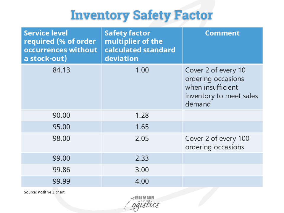
The task is to calculate the amount of safety stock required to account for variability between the quoted and actual lead times for each product or critical item. Calculate the mean and standard deviation of the cumulative lead times. The safety factor against each level of service is applied against the standard deviation to calculate the amount of safety stock, as shown in the table below.

The safety stock for a product or item provides the base to which an allowance can be added that accounts for the difference in intervals between placing orders for products or items and receiving them.

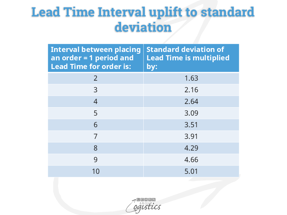
For example: If a product or item has a cumulative lead time of 8 weeks and an average sale or usage of 500 units per week, the forecast demand over the lead time is 4,000 units. However, there is a reasonable chance that demand in any of the weeks will exceed the average of 500 units, so safety stock is required. Although the safety stock must increase as the lead time increases, it is not in proportion to the increase in lead time. The table below provides the factors for adjusting the standard deviation when the lead time is not equal to the order interval:

As the availability expectation is often to provide a 98 per cent service level, the total safety inventory for a product or critical item could be more than double the safety stock required to cover only demand variability. For this reason, it requires Logisticians to have a good understanding of the service and cost implications when making and justifying decisions to minimise variability in the process and provide particular service levels as part of an inventory policy.