
Inventory budget approach by Finance
The Business Planning process, which includes budgets is typically controlled by Finance. How does Finance calculate the average value of inventory which the business can support? Is the Supply Chains group (Procurement, Operations Planning and Logistics) able to identify whether the figure provided by Finance is achievable?
The Business Planning process is discussed in the book A Framework for Supply Chains. In the Assets Plan section, the budget inventory is calculated as the Cost of Goods Sold (COGS) (also called Cost of Sales), divided by the achievable stockturn.
COGS or Cost of Sales includes purchased materials, direct labour and allocated overheads (also called burden) incurred to produce finished products (in the production process or through import). The stockturn objective is based on the prior performance of COGS divided by inventory.
One of the financial questions at the end of the Business Planning process is whether the debt to capital ratio is acceptable. If the answer is NO, Finance will adjust the numbers. To reduce the inventory budget, it is easy to increase the stockturn objective. But is there a better way to measure required inventory?
Inventory budget approach by the Supply Chains group
The overriding reason for the Supply Chains group to hold inventory is to provide Availability of products for customers. The measure of Availability is Delivery In full, On time, with Accuracy (DIFOTA). If the products are not available for delivery, DIFOTA results will be low.
The focus needs to be on the form and function of inventory by location and the inventory buffers (or safety stock) in the supply chains, that should go some way to reducing or eliminating waste. The objective is to improve forecasts and controls for fast selling SKUs and hold safety stock of low selling SKUs – the savings in inventory for fast selling SKUs will more than pay for the additional safety stock.
Analysing inventory
The ABC ranking of products, based on the Pareto or 80:20 rule, is generally known in business. However, its limitation is that all SKUs within each group are considered to have the same characteristics and behaviours and therefore can be planned in the same way. This is not correct.
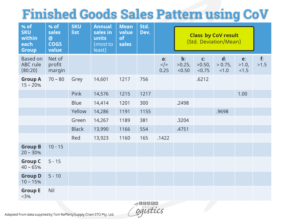
Although a group of SKUs can each have similar sales, the need is to measure the volatility in demand and assess the predictability of a demand pattern, or how well (or if at all) it can be forecast. The tool to use is the Coefficient of Variation (CoV), calculated as Coefficient of Variation = Standard Deviation / Mean.
This requires historical data of annual units sold for each SKU, listed in descending order. Sales for each SKU are in 52 weekly buckets. Calculate the mean of sales and the standard deviation. The more consistent the sales pattern of an SKU, the lower will be the CoV. For each SKU, the CoV is within a Class range of ‘a to f’ and the result placed into a table shown below. In the table, the cells Aa, Ba, Ca and Da will be within a Category that has similar patterns (and so will cells Ab, Bb, Cb and Db) and so on.
Planning inventory
From the analyse of inventory, the gains for the business come from improved planning and execution of the plan. Tom Rafferty at Supply Chain STO Pty. Ltd. has identified the range of actions to consider under the heading of CoV Management (CoVM). The table below provides an outline of Planning decision for each Category, based on CoVM.
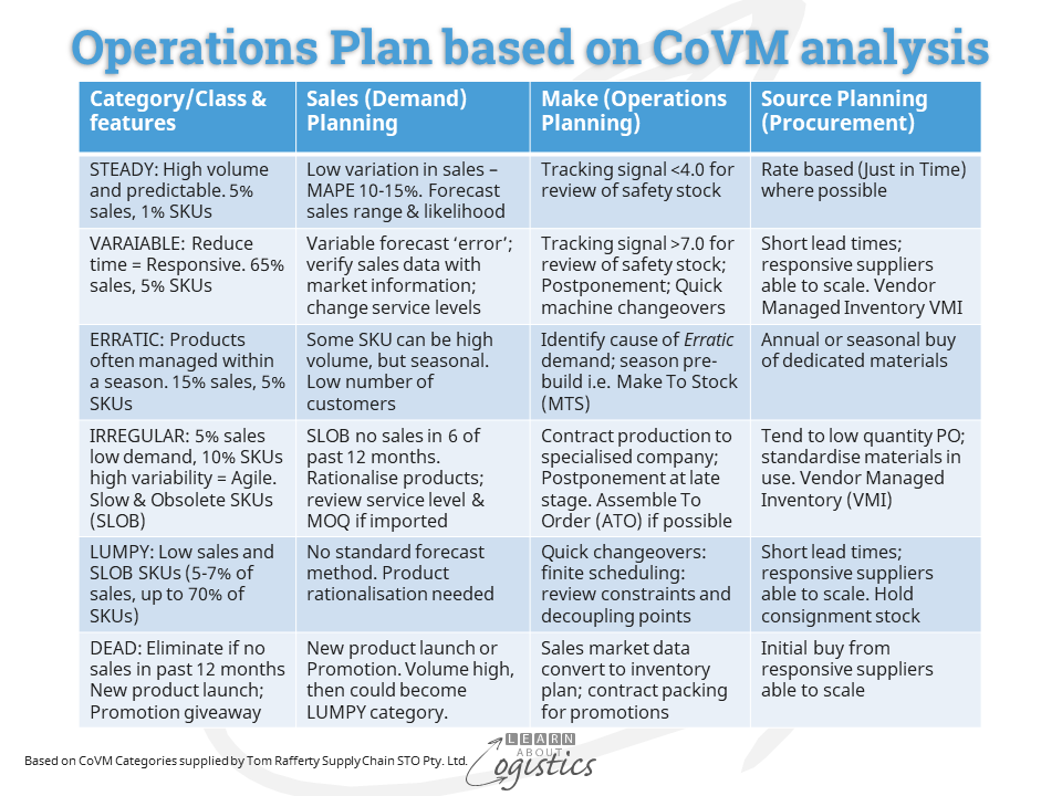
Steady (5% sales 1% SKUs): SKUs with actual sales close to forecast and with low variation. A high service level is provided with low safety stock. Measure performance with the Tracking Signal – divide the cumulative variation for the periods under review by the standard deviation. An ‘in control’ tracking signal will be less than 4.0.
Variable (65% sales, 5% SKUs): A varied forecast ‘error’ result among the SKUs. A tracking signal of >7.0 is the trigger for a review of planning for an SKU. For group/class Ac and Bc (and others if required) use a higher customer service level for safety stock calculations.
Erratic (15% sales; 5% SKUs): SKUs may have high annual sales, but sales can be highly variable by month or season. Sales are often to a small group of customers, so Logistics must work with Sales to understand the drivers of demand.
The final three patterns of demand comprise the slow and obsolete (SLOB) inventory that is often sitting in large quantities on warehouse shelves. A slow-moving SKU that has not registered any sales for six of the preceding 12 months cannot be forecast using standard time series-based forecasting methodology – instead use the Poisson probability distribution when there are infrequent demands.
Irregular (5% sales; 10-15% SKUs): SKUs are typically purchased by customers in small quantities on an irregular basis. The justification by Sales is that ‘customers demand a full range of products’. Consider different ways of obtaining and supplying these product lines e.g. contract manufacturing or Assemble to Order (ATO).
Lumpy (5-7% sales; up to 70% SKUs): This is the ‘long tail’ of SKUs. A challenge in CPG/FMCG companies is to reduce the total number of SKUs and also the introduction of more SKUs, through identifying the total costs to launch line extensions.
Service parts fit the Lumpy pattern of demand. SKUs are either for sale to customers as part of the company’s business – mainly in the automotive, defence, health and industrial equipment industries, or are used within a company’s own facilities as service parts for operational equipment e.g. a large mine site may hold over 30,000 service parts.
Dead (less than 3% SKUs): This Category covers SKUs without any sales in the past 12 months. New products and items used in promotions are included, as they do not have a sales history.
Logisticians must have a clear understanding of the service and cost implications when making (and explaining to senior management) service level decisions. For inbound supply chains, items that are directly imported are affected by varying lead time and potential delays, which require additional safety inventory. The same applies for items that are purchased from domestic suppliers, but are reliant on imported parts or ingredients.
Structuring your organisation’s inventory using the CoVM model provides a professional approach for the Supply Chains group. This can enable an agreement with Finance concerning the budget figure for inventory that recognises inventory is not a cost to be reduced but an asset to be planned.