Change in Economies

The unexpected is to be expected through supply chains. Companies that invest in mapping, monitoring and risk management for their supply chains provide a better understanding of their own capabilities to effectively respond to challenges with supply.

But what of future changes to individual economies, regions or globally? These uncertainties will occur, but when and with what severity and consequences are less certain. To help, financial and consulting firms provide economic forecasts, which, depending on their school of thought, can contain either optimistic or pessimistic outcomes based on the same inputs.

And how might changes to economies affect suppliers through the tiers of your organisation’s supply chains? There is the potential for economic changes in one or more countries to trigger events in industries and companies (at Tier 2 suppliers and below) that may have inter-dependent connections. The decisions made at lower supply tiers can affect supply and demand patterns, including your organisation’s supply.

An example is energy, primarily oil and gas, where factors outside demand and supply, such as geopolitical tensions, conflicts, trade policies of countries (including sanctions) and logistics costs are influencing prices. In turn, these can influence domestic energy prices, which may affect the future viability of companies and industries in that country.

Inventory as Time

When an economy or sales market slows in activity, an organisation’s supply chains (a complex system), begins to evolve. Existing products are updated, new products are released and old products are discontinued. But these activities may be detrimental for finished goods inventory in the sales channels or input materials that have been ordered against optimistic sales forecasts. Inventory becomes a liability because it consumes the financial liquidity of a business: it consumes physical and administrative resources and generally, the longer it is held it decreases in value.

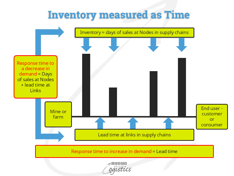
An opinion about inventory was formed in 1984, with the publication of The Goal by Goldratt & Cox. They argued that “Inventory is items purchased but not sold”…“What you do takes time and costs money. The more time it takes the more it costs. Inventory is the shadow of time. Time is a competitive measure”, as shown in the diagram below:

However, with the increase in uncertainty (and therefore risks) through supply chains , it has been argued by Taleb (who wrote The Black Swan, concerning risk) that the concept of inventory as time and therefore a cost to be avoided has created a ‘fragility’. Improving the operations of Nodes and Links in a supply chain is not enough, there must be redundancy – in capacity or inventory.

But, the strategies of outsourcing manufacturing and aiming for a high utilisation of assets has meant that the opportunity to use capacity as a buffer has generally been lost. As a result, inventory has become the critical buffer to absorb the variances between demand and supply. With this level of importance attached to inventory, there is a need to understand how (and why) your organisation’s inventory is structured. The following are elements that provide a profile of your organisation’s inventory. They have been discussed in previous blogposts.

Profile of your organisation’s inventory

In addition to the cost of holding inventory, are commitments made through purchase orders to an organisation’s suppliers (including the future supplies of outsourced manufactures). They carry the associated liabilities, even though the suppliers will not be paid until some time after delivery and acceptance, when they are shown as accounts payable. So, the inventory exposure risk exists, although it is not recorded in the accounts.

However, the Supply Chains group (Procurement, Operations Planning and Logistics) need to know the value of risk exposure as measured by Inventory Exposure, or the total amount of money committed and at risk at a given point in time. The calculation for each supply item has a cumulative lead time for purchase and subsequent steps within the business. The calculation for each supply item is Inventory Exposure = Price x Orders x Cumulative Lead-Time.

Every component part and material is required to produce and deliver a product, no matter the annual spend. But disruptions occur due to a supplier in a supply chain not receiving a low-cost item or material, which can be used across a range of products. The risk can apply equally to the supply of an item costing 10 cents or $100. The Revenue at Risk identifies the value of future sales if a Procurement risk eventuates for a purchased item. The total Revenue at Risk identifies the financial magnitude of Procurement availability risks.

Inventory Deployment identifies the structure of inventory holdings, as shown in the diagram:

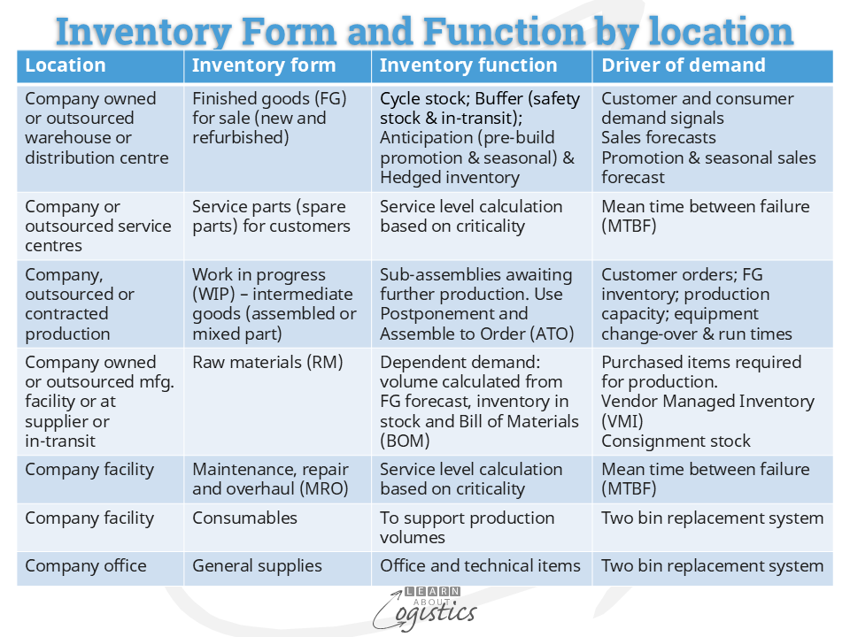
• Location: The current or intended location of an inventory SKU or supply item to meet customer service requirements and minimise stock-outs
• Form: In what form e.g. raw and packaging material; part-finished form or as a finished good and
• Function: For what inventory function – cycle, fluctuation, anticipation, in-transit (moving warehouse), hedging (seasonal or price) and ‘slow and obsolete (SLOB)
• Driver of demand

Inventory buffers are identified for Nodes in supply chains, based on the form and function of inventory.  

The Inventory Velocity (IV) measure provides a similar measure to Inventory Turns, but is calculated within the Supply Chains group. It enables a comparison of ‘stock-on-hand’ to the consumption rate and signals problems. For example, if the ‘velocity’ of SKUs slows due to excess inventory, which enhances bottlenecks, increases cycle times and affects gross margins.

The IV calculation is: Average inventory level (AIL) for a period of time/Average monthly consumption (AMC). Where AIL = OS + ((CS-OS)/2). OS = opening stock and CS = closing stock. AMC = past 12 month consumption /12. The IV is calculated for each SKU in the sales catalogue, based on 12 months of past data and the answer is expressed in ‘weeks (or days) of cover’.

The techniques discussed provide some of the base information for your organisation’s Supply Chains Design Map that identifies the necessary (and sometimes critical) information concerning the Nodes and Links in the Network.